Concept of Yield Learning¹

        In order to characterize the yield as a function of time, let us first concentrate on a single product manufacturing line. Let us also assume that only one of the pieces of equipment produces a single type of particle resulting in one type of defect. Understanding of this simplest possible case suffices to capture the essence of the yield learning process. The yield versus time curve for this scenario resembles the staircase function shown in Figure 1. 3 time variables are used.

        T_f  is the time required for analysis and detection of the failure mechanism leading to
        process intervention.

        T_e is the time needed for process correction which decreases contamination levels and the
        time required for the new process parameters to be effective.

        T_r  is the time interval after which a change in yield of the fabricated wafers is observed
        following process corrections.

        The total time required for yield change to occur is given by T_c c = (T_f  + T_e + T_r ).

        The net change in yield is Y_c . Value of Y_c  is determined by the new level of contamination.

         Estimating T_r is equivalent to estimating the cycle time for a factory albeit partially starting from an intermediate process step until the last step. Thus, it is the sum of the raw processing         time (RPT) and the queuing time for wafers waiting between process steps. One of the major contributors to the queuing time is the downtime of the equipment. Note that the factor T_e may contribute to the equipment downtime depending on the outcome of  failure analysis. T_f, the time needed to detect and localize the defect depends on a number of factors as presented in the previous chapter. The change in yield, Y_c, on the other hand depends on the correctness of the diagnosis and the efficiency with which the contamination rate can be reduced as a result of the corrective actions.

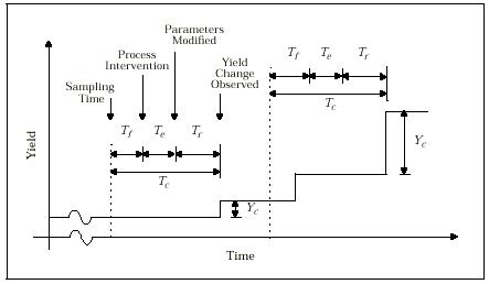
Figure¹ 1:  Key events in yield learning process.

          Thus, even for a simple factory the inter-relationship between various attributes leading to yield improvement is quite complex. Moreover a realistic situation involves a multi-product facility with more than one source of contamination, many defect  types, and several sampling and failure analysis strategies. In this case, the time to diagnose and correct different defect types will be interdependent because, for example,defects in lower layers will be "overlooked" in favor of defects in upper layers. The variability in the correctness of diagnosis will be affected since multiple sources of one type of contamination leads to ambiguity. Note that Figure 1 depicts yield improvement cycles for only one type of defect originating from one source. In reality there will be a number of such cycles overlappinging time with each other. The yield learning curve for a product is, thus, a combi-nation of all such individual overlapping learning curves.

    What Factors Affect Yield Learning?

        There are several factors that yield learning depends on.  These factors are:

            1. The relationship between particles, defects and faults.

            2. Ease of defect localization which in turn depends on:

                a. size, layer and type of defect.

                b. level of "diagnosability" of the IC design

                c. probability of occurence of catastrophic defects;

            3. Effectiveness of the corrective actions performed.

            4. The timing of each of the events mentioned above.

            5. Rate of wafer movement through the process.

        Once the fabrication line is stabilized from the point of view of global disturbances, the focus is shifted towards correcting yield loss due to local disturbances. During this stage - the yield learning stage - failed dies are analyzed and corrective actions are taken to control the level of contamination. This stage is also accompanied by an increase in the volume of production. Time domain changes in yield at this stage have a substantial impact on the cost of  manufacturing and the accrued profits. This research focuses on the defect limited yield learning for a manufacturing line. Eventually, the rate of yield learning decreases as the yield approaches 100% and this is the high volume stable  manufacturing stage. Any semiconductor manufacturing operation would like to reach this stage as quickly as possible since the bulk of the profits are realized in this period. Figure 2 shows an example average yield vs. time curve illustrating the three stages of manufacturing described above. Time domain changes in yield could also be the result of an inherent change in the nature of the disturbances, but it is mainly due to the deliberate continuous improvements made in the design and to the process. The rate of yield   learning could have been slower or faster (shown as dashed curves in Figure 2) depending on how quickly one is able to remove the process problems. A slower rate of yield learning can result not only in loss of revenue but may also lead to losing the market to other competitors.

        A higher rate of yield learning may require a more costly and complex contamination control strategy. Understanding this cost-revenue trade-off is a necessity in decision making.

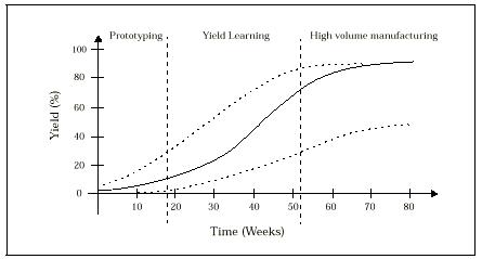
  Figure¹ 2. yield vs time curves